Comparing 2N and 4N-sized recursive segment trees

Introduction

When you implement a recursive segment tree, it’s better to store segment tree nodes in an array or vector than it is to create a new object for every node one by one. This reduces the time it takes to create the nodes and it improves caching since the nodes are in a contiguous chunk of memory.

4N implementation

If you have vector<node> nodes, you might make nodes[1] the root node and for every node x, make its left and right children 2x and 2x+1 respectively. Another way might be to have node[0] as the root and have 2x+1 and 2x+2 as the children of node x.

Either way of indexing uses $2N-1$ nodes when the segment tree is a perfect binary tree, which happens when $N$ is a power of $2$. Otherwise, we should give the tree $2 \cdot 2^{\left \lceil \log_2 N \right \rceil}$ nodes to be safe. This is because even though only $2N-1$ nodes are actually used, some indices of nodes are skipped. For convenience, we can bound this by $4N$. Our code could look something like this:

#define nm ((nl+nr)/2)

int SZ = 10; // or whatever number you need

struct node{
	// content
}; vector<node> nodes(4*SZ);

// each node nodes[rt] covers the interval [nl, nr]
void build(int nl = 0, int nr = SZ-1, int rt = 1){
	if(nl == nr){
		// initialize nodes[rt]
		return;
	}
	build(nl, nm, rt<<1);
	build(nm+1, nr, rt<<1|1);
}

2N implementations

One way to create a recursive segment tree with exactly $2n-1$ nodes is to create new nodes as we need them. As mentioned at the start, this performs far worse than the implementation with a vector of size $4n$. However, it will help us reach a solution that uses $2n$ memory. The code might look something like this:

#define nm ((nl+nr)/2)

struct node{
	// content
	node *lc, *rc;
	// lc is pointer to left child, rc is pointer to right child
};

// returns a pointer to the node that covers the interval [nl, nr]
node* build(int nl, int nr){
	node *cur = new node();
	if(nl == nr) return cur;
	cur->lc = build(nl, nm);
	cur->rc = build(nm+1, nr);
	return cur;
}

We could speed this up by creating all our nodes in advance like so:

#define nm ((nl+nr)/2)

int SZ = 10, ptr = 0;

struct node{
	// content
	int lc, rc;
	// left child is nodes[lc]
	// right child is nodes[rc]
}; vector<node> nodes(SZ*2-1);

int build(int nl, int nr){
	int cur = ptr++;
	pr(nl, nr, cur);
	if(nl == nr){
		// initialize nodes[ptr]
		return cur;
	}
	nodes[cur].lc = build(nl, nm);
	nodes[cur].rc = build(nm+1, nr);
	return cur;
}

int main(){
	build(0, 5);
}

Notice that when we are at node cur, we will assign the indices of nodes first to the left subtree, then to the right subtree. Since our recursive algorithm uses $2N’-1$ nodes to cover an interval of size $N’$, we will give the left subtree the next $2(nm-nl+1)$ nodes and give the following ones to the right subtree. This is almost the same as our original code, the only difference being how we index our nodes. This speeds up our code and uses less memory than the previous 2N implementation since we don’t need to store and check what our left and right children are.

#define nm ((nl+nr)/2)

int SZ = 10;

struct node{
	// content
}; vector<node> nodes(2*SZ-1);

void build(int nl = 0, int nr = SZ-1, int rt = 0){
	pr(nl, nr, rt);
	if(nl == nr){
		// initialize nodes[rt]
		return;
	}
	build(nl, nm, rt+1);
	build(nm+1, nr, rt+(nm-nl+1)*2);
}

Benchmarks

The question remains: is this faster than our original 4N implementation? No. In practice, the 4N implementation is faster.

Testcase	2N Segment Tree	4N Segment Tree
example_00	1 ms / 0.70 MB	1 ms / 0.61 MB
max_random_00	666 ms / 18.33 MB	653 ms / 19.11 MB
max_random_01	667 ms / 18.34 MB	649 ms / 19.09 MB
max_random_02	658 ms / 18.33 MB	654 ms / 19.09 MB
max_random_03	660 ms / 18.34 MB	652 ms / 19.08 MB
max_random_04	662 ms / 18.34 MB	653 ms / 19.09 MB
random_00	519 ms / 14.46 MB	526 ms / 18.59 MB
random_01	562 ms / 16.73 MB	560 ms / 18.71 MB
random_02	274 ms / 4.10 MB	281 ms / 4.46 MB
random_03	201 ms / 13.85 MB	203 ms / 16.84 MB
random_04	198 ms / 9.59 MB	199 ms / 17.21 MB
small_00	1 ms / 0.71 MB	1 ms / 0.71 MB
small_01	1 ms / 0.71 MB	1 ms / 0.71 MB
small_02	1 ms / 0.62 MB	1 ms / 0.71 MB
small_03	1 ms / 0.71 MB	1 ms / 0.71 MB
small_04	1 ms / 0.71 MB	1 ms / 0.71 MB

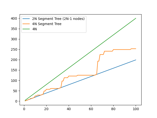
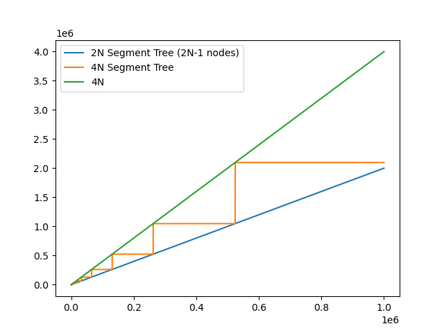
We already knew that we save up to half our memory by switching to the 2N implementation. Here is a graph of how large our vector nodes actually needs to be for each of our implementations. For the 4N implementation, our allocation of $2 \cdot 2^{\left \lceil \log_2 N \right \rceil}$ nodes was only an upper bound, albeit a reasonable one. It’s satisfying to see the 4N graph turn into a staircase as N gets large.

Memory Usage graph from 1 to 100	Memory Usage Graph from 1 to 1,000,000

Conclusions

The 2N implementation uses less memory and the 4N implementation is a little faster. These small differences will not matter if the problems you are solving have reasonable time and memory limits. If you happen to face a problem where you need to save memory or reduce the number of node merges, there is a “fat nodes” technique that I had to use exactly once.

Now of course, we could just use iterative segment trees. I guess this blog post was useless ☹️. The reason I investigated 2N vs 4N top-down segment trees was because I thought a friend’s 2N implementation was too slow.

I’d love to cover fat nodes, “walking” down iternative segment trees, and other techniques in the future. Stay tuned! 📻